

which expression results when the change of base formula is applied to ?
Author: Oscar Cronquist Article final updated on September 11, 2022
I will in this commodity demonstrate several techniques that extract or filter records based on ii conditions applied to a single column in your dataset. For example, if yous apply the array formula then the result volition refresh instantly when yous enter new start and end values.
The remaining congenital-in techniques need a lilliputian more manual work in order to use new conditions, however, they are fast. The downside with the assortment formula is that it may become slow if you lot are working with huge amounts of data.
I have too written an article in instance yous need to find records that friction match one condition in 1 column and another status in another column. The following article shows you how to build a formula that uses an arbitrary number of conditions: Extract records where all criteria lucifer if not empty
This article Excerpt records betwixt two dates is very similar to the current 1 y'all are reading right now, Excel dates are actually numbers formatted as dates in Excel. If y'all desire to search for a text cord within a given engagement range then read this article: Filter records based on a date range and a text string
I must recommend this article if you want to exercise a wildcard search across all columns in a data ready, information technology also returns all matching records. If you want to extract records based on criteria and not a numerical range then read this part of this article.
What is on this page?
- Extract all rows from a range based on range criteria (Array formula)
- Video
- How to enter an array formula
- Explaining array formula
- Extract all rows from a range based on range criteria - Excel 365
- Explaining formula
- Excerpt all rows from a range based on multiple weather (Array formula)
- Explaining array formula
- Excerpt all rows from a range based on multiple conditions - Excel 365
- Explaining formula
- Extract all rows from a range based on range critera
[Excel defined Table] - Extract all rows from a range based on range critera
[Filter] - Extract all rows from a range based on range criteria
[Avant-garde Filter] - Get Excel file
i. Extract all rows from a range based on range criteria
[Assortment formula]
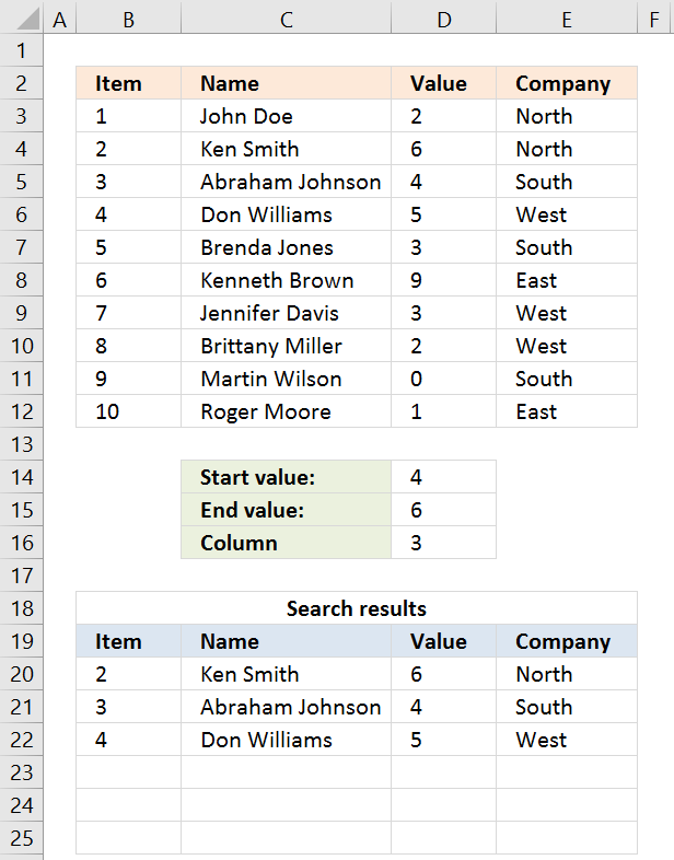
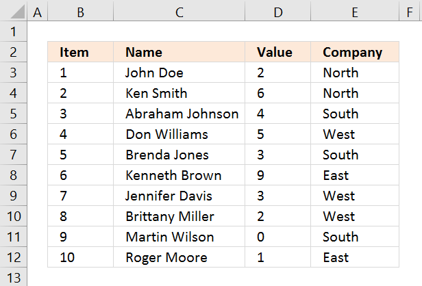
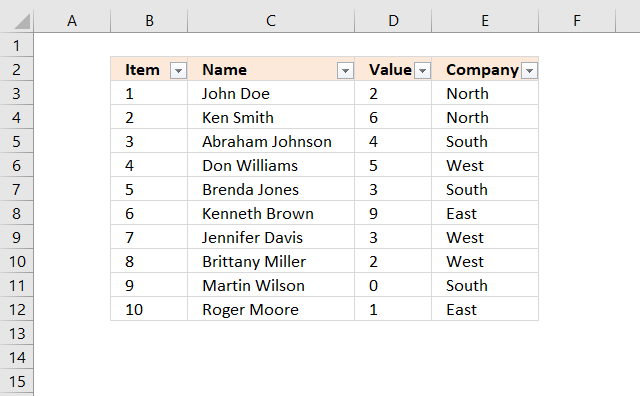
The film above shows you a dataset in cell range B3:E12, the search parameters are in D14:D16. The search results are in B20:E22.
Update 20 Sep 2022, a smaller formula in cell A20.
Array formula in cell A20:
=INDEX($B$3:$E$12, Minor(IF((INDEX($B$3:$Eastward$12, , $D$16)< =$D$15)*(Index($B$3:$E$12, , $D$sixteen)> =$D$14), MATCH(ROW($B$3:$East$12), ROW($B$three:$E$12)), ""), ROWS(B20:$B$20)), COLUMNS($A$one:A1))
Dorsum to top
one.1 Video
See this video to learn more than about the formula:
Back to top
i.two How to enter this array formula
- Select cell A20
- Paste above formula to jail cell or formula bar
- Press and hold CTRL + SHIFT simultaneously
- Press Enter once
- Release all keys
The formula bar at present shows the formula with a starting time and ending curly bracket, that is if you did the higher up steps correctly. Like this:
{=array_formula}
Don't enter these characters yourself, they appear automatically.
Now copy cell A20 and paste to cell range A20:E22.
Back to meridian
ane.3 Explaining array formula in jail cell A20
You can follow along if you select cell A19, go to tab "Formulas" on the ribbon and printing with left mouse button on the "Evaluate Formula" push button.
Step one - Filter a specific column in cell range B3:E12
The INDEX function is mostly used for getting a single value from a given cell range, notwithstanding, it tin as well return an unabridged column or row from a cell range.
This is exactly what I am doing here, the column number specified in prison cell D16 determines which column to excerpt.
INDEX($B$three:$E$12, , $D$16, ane)
becomes
INDEX($B$3:$Due east$12, , iii, ane)
and returns C3:C12.
How to use the INDEX function
Step 2 - Check which values are smaller or equal to condition
The smaller than and equal sign are logical operators that let you lot compare value to value, in this case, if a number is smaller than or equal to some other number.
The output is a boolean value, True och False. Their positions in the array represent to the positions in the jail cell range.
Index($B$iii:$Eastward$12, , $D$16, 1)< =$D$fifteen
becomes
C3:C12< =$D$xv
becomes
{two; half dozen; four; 5; 3; 9; 3; ii; 0; 1}<=half-dozen
and returns
{TRUE; True; Truthful; TRUE; TRUE; FALSE; TRUE; Truthful; Truthful; True}.
Step 3 - Multiply arrays - AND logic
There is a second status we demand to evaluate before we know which records are in range.
(INDEX($B$3:$E$12, , $D$16, 1)< =$D$fifteen)*(Index($B$3:$Eastward$12, , $D$xvi, ane)> =$D$14)
becomes
({two; vi; four; v; 3; 9; iii; 2; 0; i}< =$C$14)*({2; 6; 4; five; 3; nine; three; two; 0; 1}> =$C$13)
becomes
({2; 6; 4; v; 3; 9; 3; 2; 0; one}< =three)*({2; 6; 4; 5; iii; 9; iii; two; 0; 1}> =0)
becomes
{Truthful; FALSE; Fake; False; True; Imitation; TRUE; Truthful; True; True}*{TRUE; TRUE; True; True; TRUE; TRUE; TRUE; TRUE; TRUE; Truthful}
Both weather must be met, the asterisk lets us multiple the arrays meaning AND logic.
TRUE * True equals FALSE, all other combinations return False. True * Imitation equals Imitation and then on.
{Truthful; FALSE; Simulated; FALSE; TRUE; FALSE; True; TRUE; True; TRUE} * {TRUE; TRUE; Truthful; TRUE; TRUE; TRUE; TRUE; True; True; True}
returns
{ane; 0; 0; 0; i; 0; ane; 1; 1; one}.
Boolean values accept numerical equivalents, True = ane and False equals 0 (zero). They are converted when y'all perform an arithmetic operation in a formula.
Step 4 - Create number sequence
The ROW role calculates the row number of a cell reference.
ROW(reference)
ROW($B$3:$Due east$12)
returns
{3; four; five; 6; 7; eight; 9; ten; 11; 12}.
Stride 5 - Create a number sequence from 1 to due north
The Friction match function returns the relative position of an item in an array or prison cell reference that matches a specified value in a specific order.
Lucifer(ROW($B$iii:$Due east$12), ROW($B$3:$East$12))
becomes
Lucifer({3; iv; 5; half dozen; 7; eight; 9; 10; eleven; 12}, {iii; 4; 5; 6; vii; 8; 9; 10; 11; 12})
and returns
{ane; ii; 3; iv; 5; half-dozen; 7; 8; 9; 10}.
Pace iv - Return corresponding row number
The IF function returns one value if the logical examination is TRUE and another value if the logical examination is False.
IF(logical_test, [value_if_true], [value_if_false])
IF((Index($B$3:$E$12, , $D$sixteen)< =$D$xv)*(INDEX($B$three:$E$12, , $D$16)> =$D$14), Lucifer(ROW($B$3:$E$12), ROW($B$three:$E$12)), "")
becomes
IF({1; 0; 0; 0; 1; 0; 1; 1; 1; 1}, Friction match(ROW($B$three:$Eastward$12), ROW($B$3:$Eastward$12)), "")
becomes
IF({1; 0; 0; 0; 1; 0; ane; 1; 1; ane}, {1; two; iii; iv; 5; half dozen; 7; viii; 9; 10}, "")
and returns
{1; ""; ""; ""; five; ""; 7; 8; nine; ten}.
Step 5 - Extract one thousand-th smallest row number
The Pocket-sized function returns the m-thursday smallest value from a group of numbers.
Modest(array,one thousand)
Pocket-size(IF((Index($B$3:$E$12, , $D$16)< =$D$15)*(Alphabetize($B$3:$Eastward$12, , $D$xvi)> =$D$14), MATCH(ROW($B$3:$E$12), ROW($B$3:$East$12)), ""), ROWS(B20:$B$20))
becomes
Minor({1; ""; ""; ""; 5; ""; seven; viii; 9; 10}, ROWS(B20:$B$20))
becomes
Small-scale({1; ""; ""; ""; five; ""; 7; 8; 9; 10}, i)
and returns 1.
Step vi - Return the unabridged row record from cell range
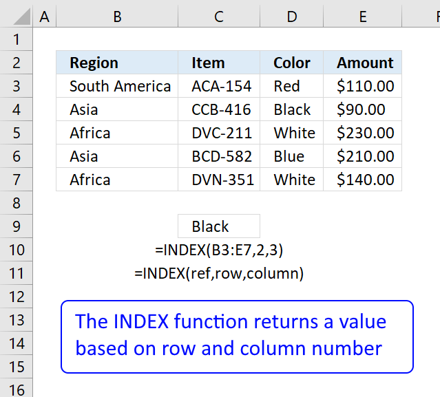
The INDEX function returns a value from a jail cell range, you specify which value based on a row and column number.
Alphabetize(assortment,[row_num],[column_num])
INDEX($B$3:$E$12, SMALL(IF((Alphabetize($B$three:$E$12, , $D$xvi)< =$D$15)*(Alphabetize($B$three:$E$12, , $D$xvi)> =$D$xiv), Lucifer(ROW($B$iii:$E$12), ROW($B$3:$E$12)), ""), ROWS(B20:$B$20)), COLUMNS($A$1:A1))
becomes
Alphabetize($B$iii:$E$12, 1, , 1)
and returns {two, "Ken Smith", 6, "Due north"}.
Recommended reading
Friction match two criteria and return multiple records
Excerpt records where all criteria match if not empty
Extract all rows that contain a value betwixt this and that
Excerpt records betwixt 2 dates
Filter records based on a engagement range and a text string
Search for a text string in a data gear up
Excerpt records containing negative values
Extract records containing digits [Formula]
Back to peak
ii. Extract all rows from a range based on range criteria - Excel 365
Update 17 December 2022,the new FILTER function is at present available for Excel 365 users. Formula in prison cell B20:
=FILTER($B$three:$Due east$12, (D3:D12<=D15)*(D3:D12>=D14))
It is a regular formula, however, it returns an array of values and extends automatically to cells beneath and to the right. Microsoft calls this a dynamic array and spilled assortment.
The array formula below is for earlier Excel versions, it searches for values that run across a range criterion (cell D14 and D15), the formula lets you change the column to search in with cell D16.
This formula can be used with whatever dataset size and shape. To search the commencement cavalcade, type 1 in cell D16.
Back to top
2.one Explaining array formula
Stride 1 - First condition
The less than character and the equal sign are both logical operators meaning they are able to compare value to value, the output is a boolean value.
In this example,
D3:D12<=D15
Step 2 - 2nd status
D3:D12>=D14
Step iii - Multiply arrays - AND logic
(D3:D12<=D15)*(D3:D12>=D14)
Step 4 - Filter values
FILTER($B$3:$E$12, (D3:D12<=D15)*(D3:D12>=D14))
Back to top
3. Extract all rows from a range that meet criteria in i column [Array formula]
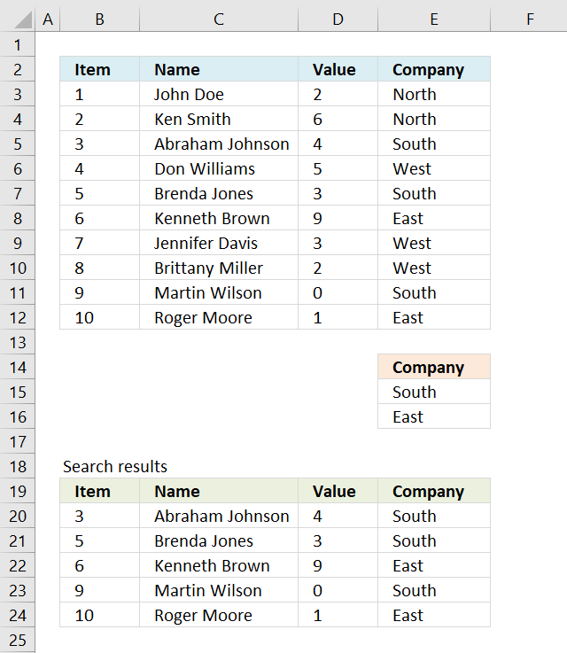
The array formula in cell B20 extracts records where column E equals either "South" or "E".
The following array formula in cell B20 is for earlier Excel versions than Excel 365:
=INDEX($B$3:$E$12, Modest(IF(COUNTIF($E$15:$E$16,$E$iii:$E$12), Lucifer(ROW($B$iii:$E$12), ROW($B$three:$Due east$12)), ""), ROWS(B20:$B$20)), COLUMNS($B$2:B2))
To enter an assortment formula, type the formula in a cell then press and concur CTRL + SHIFT simultaneously, now press Enter one time. Release all keys.
The formula bar now shows the formula with a beginning and ending curly bracket telling you that you entered the formula successfully. Don't enter the curly brackets yourself.
Dorsum to top
3.i Explaining formula in cell B20
Step 1 - Filter a specific column in cell range $A$2:$D$11
The COUNTIF function allows yous to identify cells in range $East$iii:$E$12 that equals $E$15:$E$xvi.
COUNTIF($E$15:$E$16,$Due east$3:$East$12)
becomes
COUNTIF({"S"; "East"},{"North"; "North"; "S"; "Westward"; "South"; "East"; "West"; "West"; "South"; "Due east"})
and returns
{0;0;1;0;one;i;0;0;ane;1}.
Step 2 - Return corresponding row number
The IF function has three arguments, the kickoff one must be a logical expression. If the expression evaluates to True and then one thing happens (argument ii) and if Faux some other affair happens (argument 3).
The logical expression was calculated in step one , True equals i and Faux equals 0 (naught).
IF(COUNTIF($Eastward$15:$E$16,$E$iii:$E$12), MATCH(ROW($B$3:$E$12), ROW($B$three:$E$12)), "")
becomes
IF({0; 0; 1; 0; one; ane; 0; 0; 1; 1}, MATCH(ROW($B$iii:$Due east$12), ROW($B$3:$E$12)), "")
becomes
IF({0; 0; 1; 0; 1; 1; 0; 0; 1; one}, {one; 2; 3; 4; v; half-dozen; 7; eight; ix; 10}, "")
and returns
{""; ""; 3; ""; 5; 6; ""; ""; 9; 10}.
Step 3 - Observe yard-th smallest row number
SMALL(IF(COUNTIF($E$15:$E$16,$East$3:$Due east$12), MATCH(ROW($B$3:$E$12), ROW($B$iii:$Due east$12)), ""), ROWS(B20:$B$20))
becomes
Small-scale({""; ""; three; ""; v; six; ""; ""; 9; 10}, ROWS(B20:$B$20))
becomes
Pocket-sized({""; ""; iii; ""; 5; 6; ""; ""; ix; 10}, ane)
and returns iii.
Footstep four - Return value based on row and column number
The INDEX function returns a value based on a jail cell reference and column/row numbers.
Alphabetize($B$3:$E$12, Small-scale(IF(COUNTIF($E$15:$Due east$xvi,$East$3:$E$12), MATCH(ROW($B$3:$E$12), ROW($B$iii:$E$12)), ""), ROWS(B20:$B$xx)), COLUMNS($B$two:B2))
becomes
Alphabetize($B$3:$E$12, 3, COLUMNS($B$2:B2))
becomes
INDEX($B$three:$E$12, 3, 1)
and returns 3 in cell B20.
Back to top
Recommended reading
- Lucifer 2 criteria and render multiple records
- Extract records where all criteria match if not empty
- Extract all rows that contain a value between this and that
- Excerpt records between two dates
- Filter records based on a date range and a text string
- Search for a text cord in a data gear up
- Extract records containing negative values
- Excerpt records containing digits [Formula]
Back to top
4. Excerpt all rows from a range based on multiple conditions - Excel 365
Update 17 Dec 2022,the new FILTER part is at present available for Excel 365 users. Formula in cell B20:
=FILTER($B$3:$East$12, COUNTIF(E15:E16, E3:E12))
It is a regular formula, all the same, it returns an assortment of values. Read here how it works: Filter values based on criteria
The formula extends automatically to cells below and to the correct. Microsoft calls this a dynamic assortment and spilled assortment.
Back to elevation
4.1 Explaining array formula
Step ane -
COUNTIF(E15:E16, E3:E12)
Stride 2 -
FILTER($B$three:$E$12, COUNTIF(E15:E16, E3:E12))
Back to peak
5. Extract all rows from a range that run across criteria in one column [Excel defined Tabular array]
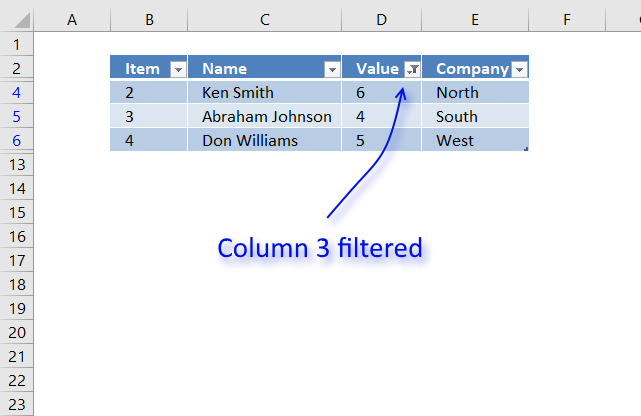
The image above shows a dataset converted to an Excel defined Table, a number filter has been applied to the third column in the table.
Hither are the instructions to create an Excel Table and filter values in column 3.
- Select a jail cell in the dataset.
- Press CTRL + T
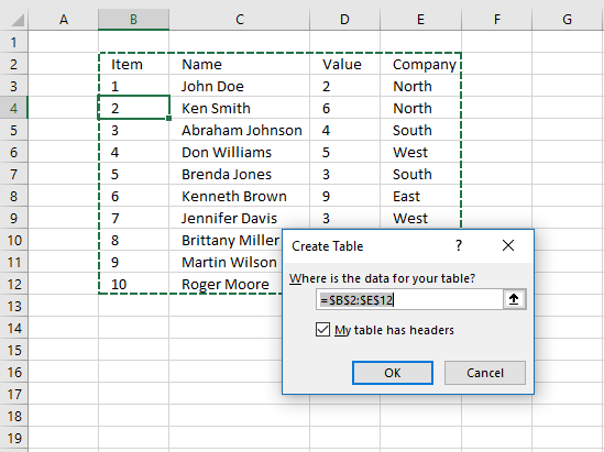
- Printing with left mouse button on check box "My tabular array has headers".
- Press with left mouse button on OK button.

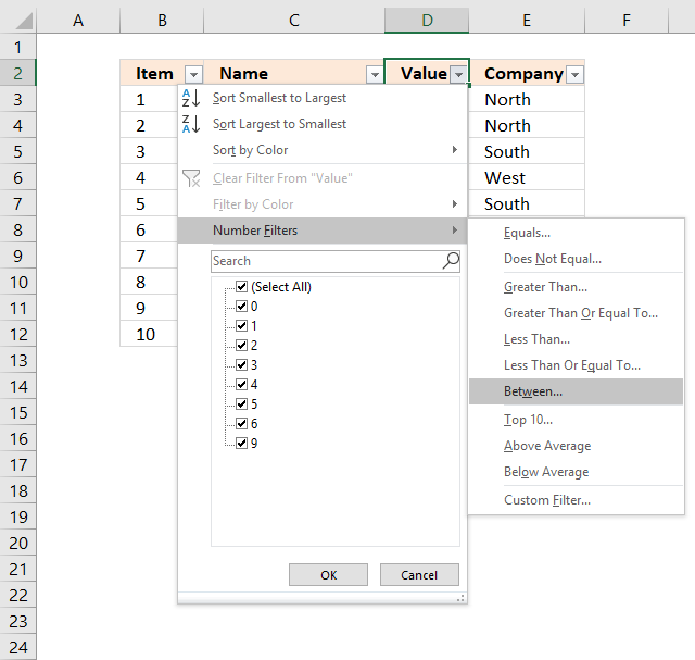
The paradigm in a higher place shows the Excel defined Table, here is how to filter D betwixt four and half dozen:
- Printing with left mouse button on black arrow next to header.
- Printing with left mouse button on "Number Filters".
- Press with left mouse push on "Between...".
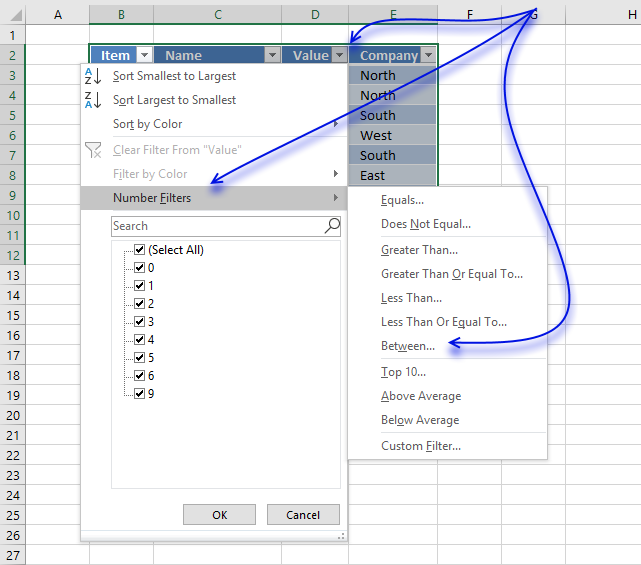
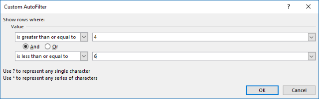
- Blazon 4 and 6.

- Printing with left mouse push on OK button.
Back to top
6. Extract all rows from a range that see criteria in i column [Filter]
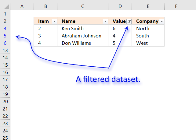
The prototype above shows filtered records based on two conditions, values in column D are larger or equal to iv or smaller or equal to 6.
Hither is how to utilize Filter arrows to a dataset.
- Select any cell inside the dataset range.
- Go to tab "Data" on the ribbon.
- Press with left mouse button on "Filter push button".
Black arrows appear adjacent to each header.
Lets filter records based on conditions applied to column D.
- Press with left mouse button on blackness arrow next to header in Column D, run across image below.
- Printing with left mouse button on "Number Filters".
- Printing with left mouse push on "Between".
- Type 4 and six in the dialog box shown beneath.
- Printing with left mouse button on OK button.
Back to top
7. Extract all rows from a range that meet criteria in i column
[Avant-garde Filter]
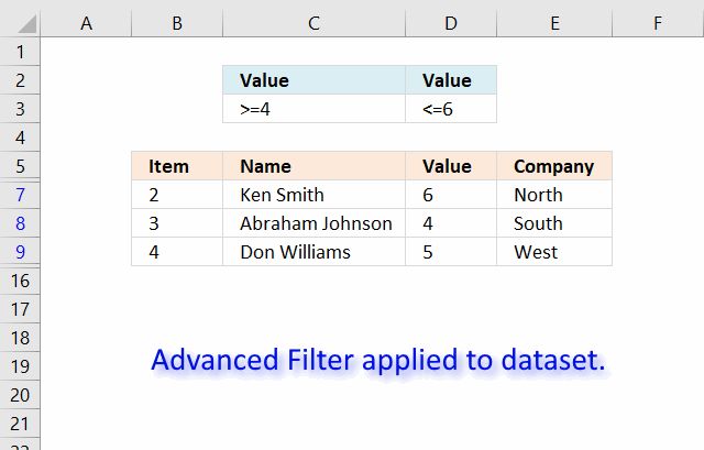
The image above shows a filtered dataset in cell range B5:E15 using Advanced Filter which is a powerful feature in Excel.
Here is how to use a filter:
- Create headers for the column you lot desire to filter, preferably above or below your data set.
Your filters will mayhap disappear if placed next to the data fix because rows may become hidden when the filter is applied. - Select the unabridged dataset including headers.
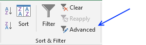
- Go to tab "Data" on the ribbon.
- Press with left mouse button on the "Advanced" button.
- A dialog box appears.
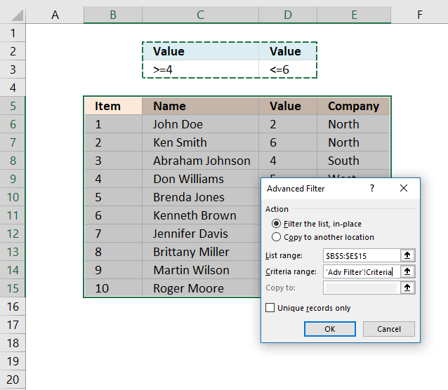
- Select the criteria range C2:D3, shown ithe northward above paradigm.
- Press with left mouse button on OK button.
Back to tiptop
Recommended posts
Read this mail service and come across how to extract indistinguishable records:
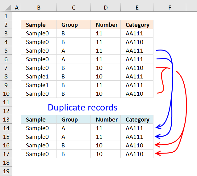
Extract duplicate records
This article describes how to filter indistinguishable rows with the apply of a formula. It is, in fact, an array […]
Extract duplicate records
Learn how to filter unique singled-out records:
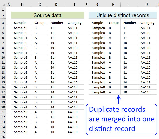
Filter unique distinct records
Table of contents Filter unique singled-out row records Filter unique singled-out row records but not blanks Filter unique distinct row […]
Filter unique distinct records
Dorsum to pinnacle
8. Excel file

Source: https://www.get-digital-help.com/extract-all-rows-from-a-range-that-meet-criteria-in-one-column-in-excel/
Posted by: leavellanchey86.blogspot.com
0 Response to "which expression results when the change of base formula is applied to ?"
Post a Comment